Historic Volatility
Consider the following parameters:
· Si: stock price at end of ith interval, i = 0, 1, …, n
· τ: length of time interval in years
· xi: return on stock over ith interval in percent
· xavg: mean of the returns xi
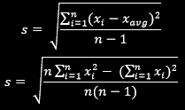
· s: standard deviation of xi in percent
Given the stock prices at the end of the ith intervals (Si), we compute the returns on the stock over the ith intervals (i = 1, 2, …, n) using one of the following two conventions:
· Standard Returns:
Consider the following parameters:
· Si: stock price at end of ith interval, i = 0, 1, …, n
· τ: length of time interval in years
· xi: return on stock over ith interval in percent
· xavg: mean of the returns xi
· s: standard deviation of xi in percent
Given the stock prices at the end of the ith intervals (Si), we compute the returns on the stock over the ith intervals (i = 1, 2, …, n) using one of the following two conventions:
· Standard Returns:
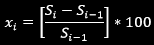
· Logarithmic Returns:
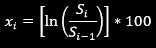
After computing the returns stream, we compute the standard deviation of returns as follows:
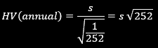
Annual Historic Volatility can thus be written as: HV(annual) = s / √ τ
For instance, if historic data was gathered on a daily basis, then τ = 1/252 and Historic Volatility would be:
For instance, if historic data was gathered on a daily basis, then τ = 1/252 and Historic Volatility would be:
Implied Volatility
This procedure offers an estimate of price volatility which is derived from the market price of an option. Calculations are conducted until the volatility of the model gives a price that lies within a predetermined margin error ε (0.00001) of the instrument’s actual market price. The option pricing model used is the Black-Scholes continuous-time model for pricing European options.
Consider the following parameters (as inputs to the model):
· Underlying/Stock price
· Option strike/exercise price
· Continuously compounded risk-free rate in percent
· Option price
· Option term/maturity in years
· Type of option (European Call/Put)
The procedure consists of starting off with a volatility of 100%, and calculating the corresponding option price. If the calculated price (at 100%) is lower than the target price, the second step would be to take a jump up to 200% and compare the price at that level to the target. We keep on incrementing the volatility to test with by a factor of two on the way up (and adjusting our bounds accordingly) until the calculated price is higher than the target price, at which point we test on the volatility midway between our bounds (midpoint of our bounding window) and carry on the process recursively.
If the calculated price (at 100%) is higher than the target price, the second step would be to take a jump down to 50% and compare the price at that level to the target. We keep on decrementing the volatility to test with by a factor of half on the way down (and adjusting our bounds accordingly) until the calculated price is lower than the target price, at which point we test on the volatility midway between our bounds (midpoint of our bounding window) and carry on the process recursively.
Our volatility generating method keeps on going back and forth in an attempt to capture the target option price until we establish a bounding window of ε (0.00001), at which the method comes to a stop and the volatility at the midpoint of the lastly established bounding window is output.
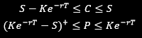
Bounds
The module requires the input parameters to be within a set of pre-specified bounds. These bounds are checked, and the user is made aware of any invalid entries before passing the parameters on to the function (for volatility calculation), as to avoid any undesirable outputs.
Bounds on European Call/Put options: