Binomial Pricing
Consider the following relevant parameters:
· σ: asset’s annualized volatility (in percent)
· ∆t: (option term/number of binomial steps) –time period (in years) in binomial model
· δ: (Annual dividend percent * ∆t) –dividend payment at each binomial step (in percent)
· u: exp(σ√∆t) –factor by which stock is expected to increase over one period
· d: exp(-σ√∆t) –factor by which stock is expected to decrease over one period
· R: 1+rf –one period return on the risk-free asset
· q: (R-d)/(u-d) –risk-neutral probability
· Zi: derivative payoff at stage ‘i’ of binomial model (Z typically being a Call-C, or Put-P)
· K: option strike price
· S0: current stock/underlying price
Given σ and ∆t, we compute u and d. We then compute the option payoff at maturity, and work backwards using the risk-neutral probability to compute the option prices at earlier stages of the model to reach the current arbitrage free option price.
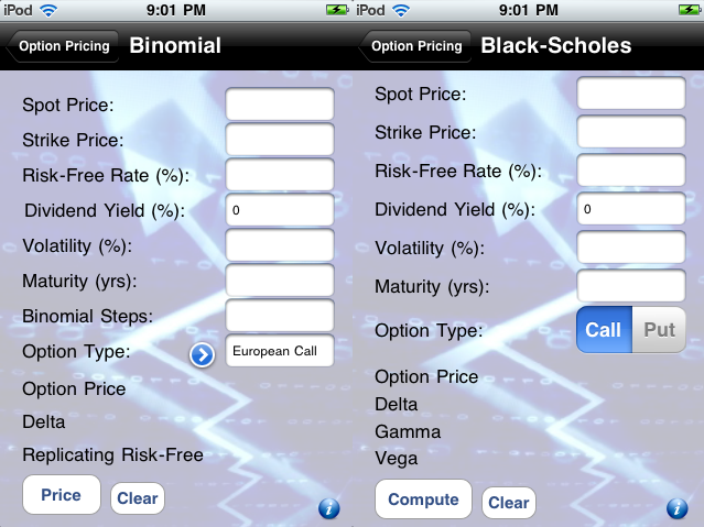
The user would be prompt to input: (1) Underlying Current/Spot Price S0, (2) Strike price K, (3) Annual Risk-Free rate rf (in percent), (4) Annual dividend payments (in percent), (5) Underlying Price Volatility σ (in percent), (6) Option Term/Maturity T (in years), (7) Number of Binomial steps N, and (8) Type of Option (European Call/Put, American Call/Put).
European Call Example:
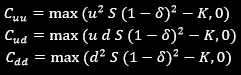
We work out an example with a European Call option on a 3-period binomial model:The value of the option is known at the final node of the lattice:
Consider the following relevant parameters:
· σ: asset’s annualized volatility (in percent)
· ∆t: (option term/number of binomial steps) –time period (in years) in binomial model
· δ: (Annual dividend percent * ∆t) –dividend payment at each binomial step (in percent)
· u: exp(σ√∆t) –factor by which stock is expected to increase over one period
· d: exp(-σ√∆t) –factor by which stock is expected to decrease over one period
· R: 1+rf –one period return on the risk-free asset
· q: (R-d)/(u-d) –risk-neutral probability
· Zi: derivative payoff at stage ‘i’ of binomial model (Z typically being a Call-C, or Put-P)
· K: option strike price
· S0: current stock/underlying price
Given σ and ∆t, we compute u and d. We then compute the option payoff at maturity, and work backwards using the risk-neutral probability to compute the option prices at earlier stages of the model to reach the current arbitrage free option price.
The user would be prompt to input: (1) Underlying Current/Spot Price S0, (2) Strike price K, (3) Annual Risk-Free rate rf (in percent), (4) Annual dividend payments (in percent), (5) Underlying Price Volatility σ (in percent), (6) Option Term/Maturity T (in years), (7) Number of Binomial steps N, and (8) Type of Option (European Call/Put, American Call/Put).
European Call Example:
We work out an example with a European Call option on a 3-period binomial model:The value of the option is known at the final node of the lattice:
We define the risk-neutral probability as: q = (R - d) / (u - d)
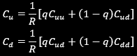
We find the values of Cu and Cd:
We find the values of Cu and Cd:
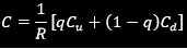
We then find C by another application of the same risk-neutral discounting formula:
Hedging Strategy:
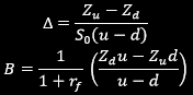
Hedging Strategy or Replicating Strategy approach aims at replicating the option’s payoff /value at each stage throughout the binomial lattice. It consists of forming a portfolio with ∆ units of the underlying (stock) and $B worth of riskless bond. We pick portfolio weights to match the derivative payoffs:
“up”: ∆uS0 + (1 + rf)B = Zu
“down”: ∆dS0 + (1 + rf)B = Zd
Solving the above system of two equations in two unknowns, we get:
We have the module output the replicating portfolio weights ∆ and B for the underlying and riskless bond respectively for the very first step of the binomial lattice.
Black-Scholes Model
The Black-Scholes model is a continuous-time model developed to price European options based on a number of assumptions:
· Stock prices follow a random walk
· Volatility is constant
· No transactions costs or taxes
· Continuous trading
· No limits on short-selling
· Constant interest rate
The model takes the following parameters as inputs:
· S = stock price
· K = option strike/exercise price
· T = option term/maturity (in years)
· r = continuously compounded annual risk-free rate (in percent)
· σ = stock volatility (in percent)
· δ = continuously paid annual dividends (in percent)
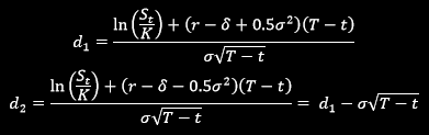
The Black-Scholes formula for the value of a European call option on a non-dividend paying stock is given by:
Black-Scholes Model
The Black-Scholes model is a continuous-time model developed to price European options based on a number of assumptions:
· Stock prices follow a random walk
· Volatility is constant
· No transactions costs or taxes
· Continuous trading
· No limits on short-selling
· Constant interest rate
The model takes the following parameters as inputs:
· S = stock price
· K = option strike/exercise price
· T = option term/maturity (in years)
· r = continuously compounded annual risk-free rate (in percent)
· σ = stock volatility (in percent)
· δ = continuously paid annual dividends (in percent)
The Black-Scholes formula for the value of a European call option on a non-dividend paying stock is given by:

where N(x) denotes the standard cumulative normal probability distribution.
Put-call parity gives the put price: